

To investigate the phenomena of a transformer inrush current, the basics of transformer analysis has to be understood together with basics of magnetism explained in this post. To simplify the analysis, we analyse the ideal transformer. The ideal transformer core saturation is neglected and the permeability of iron (or steel) is considered constant.
Lumped elements
On the fig.1 the simplified equivalent circuit of transformer is shown with linear elements. The values of copper (winding) resistances R and a reactance X from leakage flux (the magnetic flux that does not close through the iron core, rather through the air between windings or the transformer housing) are referred to the primary side with factor a which is the ratio of turns between primary and secondary side:


The transformer is connected to a strong grid with sinusoidal voltage (we will consider that transformer circuit does not influence the voltage of the strong grid):

The secondary of the transformer is the open circuit. Therefore, when the grid voltage is applied to the transformer as a primary voltage, the current that will flow through a primary winding will be the current that establishes a magnetic field and a magnetic flux in the core and a magnetic flux leaking in the air. Understanding the circuit, we can conclude that:

By applying Ohm’s law on the primary contour, the next differential equation emerges:

where 
- Transient part – the part that decays over time if the system damping is positive
- Steady state part – the part that is the product by input function excitation
The solution for our application is following:

where 


Multiple conclusions are drawn here:
- The decaying time of transient part of the current is dependent on transformer design and partly on the system where the transformer is connected. The higher resistance, the faster the decay will be. The higher inductance, the oscillations will last longer.
- The value of the current cannot be changed instantaneously due to the inductance. Before the energization of a transformer at time
, the current is not flowing. After connecting the voltage to the primary at time
the current has to start from the value of zero. For value
to be zero, the components
and
have to both be zero or they have to have same magnitude but opposite sign.
- By changing the energizing time, the voltage angle
- If the transformer is energized at the time that voltage is maximum i.e.
, the transient part of the current will not exist since
.
- If the transformer is energized at the time that voltage is minimum i.e.
, the transient part of the current will have the same magnitude as steady state because
. The resulting current i(t) will reach the almost the twice the value at the first peak due to the energizing time.
- If the transformer is energized at the time that voltage is maximum i.e.
Magnetic circuit analysis
The other approach to the presented conclusions can be shown by an equivalent magnetic circuit of a transformer. As a first step, all the relations are linear and the material saturation is neglected. According to a Faraday’s law, the induced voltage over the primary winding when external voltage source is applied is given with the relation:

where 


To calculate the 

If the transformer was energized in the past the remanent flux is still present in the transformer core. The reason behind this is the nature of hysteresis of BH curve. If the strength of magnetic field is reduced to the zero, i.e. the magneto-motive force is reduced to the zero, the flux density does not disappear. According to the domain theory, after removing the H some of the domains are still oriented as the magnetic field that was present. That value is dependent on the material and it is labeled 

Important notice is that the magnetic flux cannot be changed instantaneously, similar to the current. It is obvious that depending on the energizing angle

We can analyse two marginal cases when transformer is energized when the voltage is at its zero (


- Voltage at the zero crossing
- Voltage at the positive maximum


As explained in this post, for the linear characteristic that we assumed, the flux is proportional to the magnetizing current. Therefore, for energizing the transformer at the time that voltage is maximum i.e. 

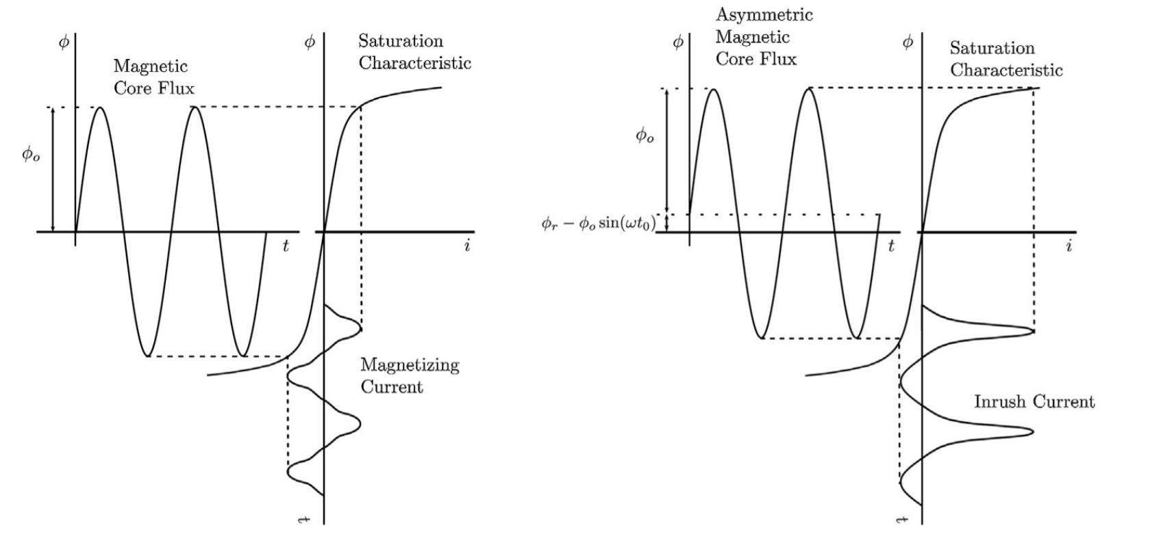
The BH curve
By introducing the BH curve into our analysis, the complete picture of inrush current is drawn. The property of the material is that it will get saturated at the specified point. In other words, the current in magneto-motive force needed to produce an increase in magnetic flux 

One has to bear in mind that this is one phase analysis. For the three phase transformer, the story is similar (depends a bit on the type of the core). If three phases are energized at the same time, there will be always some inrush magnetization current because there is no moment in which all three phase symmetrical voltages are at its maximum. So more advanced techniques have to be implemented to reduce large inrush currents. Also, the remanent flux in the three phase transformer is not the same in all phases since the flux was different for the each phase prior to disconnection.

